

ratwolf
Bronze Coder
GitHub
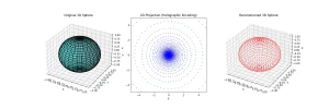
The stereographic projection offers a fascinating analogy for understanding emergent dimensions — the idea that higher-dimensional information can be encoded in a lower-dimensional surface. While not a direct physical model, it helps visualize how the third dimension of spacetime might not be fundamental, but instead an emergent property arising from a deeper 2D description.
The Power of Stereographic Projection
This mathematical technique maps points from a 3D sphere onto a
2D plane, demonstrating how three-dimensional data can be represented in fewer dimensions. Crucially, the projection is reversible — meaning the original 3D structure can be perfectly reconstructed from its 2D counterpart.
Stereographic Projection Formula
For a unit sphere S^2 centered at the origin in 3D space with coordinates x, y, z, the stereographic projection onto the xy plane is given by:
Code:
   x' = x / (1 - z)
   y' = y / (1 - z)
where x', y' are the coordinates of the projected point on the 2D plane.
Inverse Stereographic Projection
To recover the 3D coordinates from the 2D projection, we use the inverse stereographic projection:
Code:
   x = 2x' / (1 + x'^2 + y'^2)
   y = 2y' / (1 + x'^2 + y'^2)
   z = (1 - x'^2 - y'^2) / (1 + x'^2 + y'^2)
This reversibility illustrates how higher-dimensional information can be encoded and decoded in a lower-dimensional framework — an essential concept in theories of emergent spacetime.
From Math to Physics: The Emergent Dimension Analogy
The stereographic projection serves as a classical geometric analogy for the holographic principle, which suggests that our 3D universe might be encoded on a 2D boundary. However, this is just an illustration — the real holographic principle in quantum gravity involves far deeper mechanisms, such as:
- Quantum entanglement
- Boundary conformal field theories
- Non-local information encoding
Still, the stereographic projection provides valuable intuition for how extra dimensions could emerge from simpler structures.
Why This Matters
By studying such projections, we gain insight into how:
- Higher-dimensional physics might arise from lower-dimensional rules.
- Spacetime itself could be an emergent phenomenon.
- Quantum gravity theories (like AdS/CFT*) use holographic encoding.
While the full picture requires advanced quantum theory, the stereographic projection offers a beautiful geometric gateway into these profound ideas.
Python:
import numpy as np
import matplotlib.pyplot as plt
from mpl_toolkits.mplot3d import Axes3D

# Generate a 3D sphere
theta = np.linspace(0, np.pi, 30)
phi = np.linspace(0, 2 * np.pi, 60)
theta, phi = np.meshgrid(theta, phi)

# Convert spherical coordinates to Cartesian (3D)
x = np.sin(theta) * np.cos(phi)
y = np.sin(theta) * np.sin(phi)
z = np.cos(theta)

# Stereographic Projection (3D -> 2D)
x_proj = x / (1 - z)
y_proj = y / (1 - z)

# Inverse Projection (2D -> 3D)
x_recon = (2 * x_proj) / (1 + x_proj**2 + y_proj**2)
y_recon = (2 * y_proj) / (1 + x_proj**2 + y_proj**2)
z_recon = (1 - x_proj**2 - y_proj**2) / (1 + x_proj**2 + y_proj**2)

# Create figure with 3 subplots
fig = plt.figure(figsize=(18, 6))

# --- Original 3D Sphere ---
ax1 = fig.add_subplot(131, projection='3d')
ax1.plot_surface(x, y, z, color='cyan', edgecolor='black', alpha=0.3)
ax1.set_title("Original 3D Sphere")
ax1.set_xlabel("X")
ax1.set_ylabel("Y")
ax1.set_zlabel("Z")

# --- 2D Stereographic Projection (Emergent Dimension Encoding) ---
ax2 = fig.add_subplot(132)
ax2.scatter(x_proj, y_proj, s=1, color='blue')
ax2.set_title("2D Projection (Holographic Encoding)")
ax2.set_xlabel("X'")
ax2.set_ylabel("Y'")
ax2.set_xlim([-5, 5])
ax2.set_ylim([-5, 5])
ax2.set_aspect('equal')

# --- Reconstructed 3D Sphere ---
ax3 = fig.add_subplot(133, projection='3d')
ax3.scatter(x_recon, y_recon, z_recon, s=1, color='red')
ax3.set_title("Reconstructed 3D Sphere")
ax3.set_xlabel("X")
ax3.set_ylabel("Y")
ax3.set_zlabel("Z")

plt.show()
Advanced version:
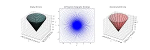
Python:
import numpy as np
import matplotlib.pyplot as plt
from mpl_toolkits.mplot3d import Axes3D

def parametric_surface(u, v, shape):
    """
    Generate parametric surface based on user selection.
    """
    if shape == "sphere":
        x = np.sin(u) * np.cos(v)
        y = np.sin(u) * np.sin(v)
        z = np.cos(u)
    elif shape == "cone":
        k = 1  # Cone slope
        r = u
        x = r * np.cos(v)
        y = r * np.sin(v)
        z = k * r
    elif shape == "paraboloid":
        r = u
        x = r * np.cos(v)
        y = r * np.sin(v)
        z = r ** 2  # Parabolic height
    else:
        raise ValueError("Unknown shape: Choose 'sphere', 'cone', 'paraboloid'")
    return x, y, z

def stereographic_projection(x, y, z):
    """
    Apply stereographic projection from the north pole (z = 1).
    """
    with np.errstate(divide='ignore', invalid='ignore'):
        x_proj = x / (1 - z)
        y_proj = y / (1 - z)
    return x_proj, y_proj

def inverse_projection(x_proj, y_proj, shape):
    """
    Reconstruct 3D surface based on original shape equation.
    """
    r_proj = np.sqrt(x_proj**2 + y_proj**2)
    phi_proj = np.arctan2(y_proj, x_proj)

    if shape == "sphere":
        denom = 1 + r_proj**2
        x_recon = (2 * x_proj) / denom
        y_recon = (2 * y_proj) / denom
        z_recon = (1 - r_proj**2) / denom
    elif shape == "cone":
        x_recon = x_proj
        y_recon = y_proj
        z_recon = np.sqrt(x_proj**2 + y_proj**2)  # Matching cone equation
    elif shape == "paraboloid":
        x_recon = x_proj
        y_recon = y_proj
        z_recon = x_proj**2 + y_proj**2  # Matching paraboloid equation

    else:
        raise ValueError("Unknown shape: Choose 'sphere', 'cone', 'paraboloid', or 'ellipsoid'.")

    return x_recon, y_recon, z_recon

# Select shape
shape_type = "cone"  # Change this to test different shapes

# Generate a parametric surface
u_res, v_res = 190, 100  # Increased resolution
u = np.linspace(0, np.pi, u_res) if shape_type == "sphere" else np.linspace(0, 1, u_res)
v = np.linspace(0, 2 * np.pi, v_res)
u, v = np.meshgrid(u, v)

x, y, z = parametric_surface(u, v, shape_type)

# Apply stereographic projection
x_proj, y_proj = stereographic_projection(x, y, z)

# Reconstruct the surface using inverse projection
x_recon, y_recon, z_recon = inverse_projection(x_proj, y_proj, shape_type)

# Explicitly close the grid by appending the first row to the end
x_recon = np.vstack([x_recon, x_recon[0, :]])
y_recon = np.vstack([y_recon, y_recon[0, :]])
z_recon = np.vstack([z_recon, z_recon[0, :]])

# Create figure with 3 subplots
fig = plt.figure(figsize=(18, 6))

# --- Original 3D Surface ---
ax1 = fig.add_subplot(131, projection='3d')
ax1.plot_surface(x, y, z, color='cyan', edgecolor='black', alpha=0.3)
ax1.set_title(f"Original 3D {shape_type.capitalize()}")
ax1.set_xlabel("X")
ax1.set_ylabel("Y")
ax1.set_zlabel("Z")

# --- 2D Projection ---
ax2 = fig.add_subplot(132)
ax2.scatter(x_proj, y_proj, s=1, color='blue')
ax2.set_title("2D Projection (Holographic Encoding)")
ax2.set_xlabel("X'")
ax2.set_ylabel("Y'")
ax2.set_xlim([-5, 5])
ax2.set_ylim([-5, 5])
ax2.set_aspect('equal')

# --- Reconstructed 3D Surface ---
ax3 = fig.add_subplot(133, projection='3d')

# Choose between coarse surface grid or wireframe
visualization_mode = "coarse_grid"  # Change to "coarse_grid" for coarse surface grid

if visualization_mode == "coarse_grid":
    # Coarse surface grid
    ax3.plot_surface(x_recon, y_recon, z_recon, color='red', edgecolor='black', alpha=0.3, rstride=5, cstride=5)
elif visualization_mode == "wireframe":
    # Wireframe
    ax3.plot_wireframe(x_recon, y_recon, z_recon, color='red', rstride=5, cstride=5)
else:
    raise ValueError("Unknown visualization mode: Choose 'coarse_grid' or 'wireframe'")

ax3.set_title(f"Reconstructed 3D {shape_type.capitalize()}")
ax3.set_xlabel("X")
ax3.set_ylabel("Y")
ax3.set_zlabel("Z")

plt.show()
Last edited: